Application of the steady laminar flamelet model for humidified non-premixed swirl flames: effects of water vapor addition on nox emissions

Abstract

Introduction

Combustion is a method of energy conversion, and turbulence is fundamental to increasing efficiency and reducing pollutant emissions. In recent years, several models that address the coupling between turbulence and the kinetic chemistry of oxidation have been developed and integrated into numerical codes for computational fluid simulation.
The most popular models are the eddy dissipation model (EDM), the eddy dissipation concept (EDC), chemical equilibrium (CE), flamelet models, the flamelet-generated manifold (FGM), and the transported probability density function (T-PDF) approach [1, 2].
The flamelet model has become essential in the numerical simulation of turbulent combustion flames due to its ability to combine detailed turbulence and chemical kinetics within the flame structure. This model was initially developed in the 1970s [3] and has been successfully applied to various types of flames.
A key advantage of this model lies in its ability to provide reliable predictions of temperature and chemical composition fields without directly solving all the transport equations for the chemical species, while simultaneously reducing computational cost and preserving the influence of detailed chemical kinetics and mixture fraction gradients.
Given that the flamelet model is widely used in large eddy simulations (LES) [4–7], the same model has generally adapted well and appears effective in modeling with the Reynolds statistical averaging method [8–10].
Several studies have investigated the structure of the flame and even the formation of NOx using this model, and some examples include [12–16]. The advantage of the SLF model compared to the EDC model is that the flamelet model does not require a high-quality mesh, which means that for more complex geometries, or where further refinement is needed in specific areas, the SLF model is better suited to these geometries and does not require additional refinement.
 

We chose the BERL combustion chamber configuration because it represents a real-world case that links laboratory research with industrial applications. This combustion chamber is known experimentally, or its measurement data is freely accessible. The flame developing inside this chamber serves to validate our calculation. The data from the IFRF experimental studies referenced in [17] and the numerical calculations referenced in [18-20] provide important data for validating our calculations. We can cite some studies based on the effect of using detailed chemical kinetic mechanisms on the evolution of flame temperature as well as on its speed [21–24].
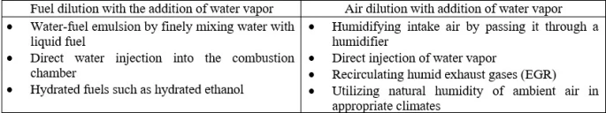
All research on the phenomenon of turbulent combustion in various industrial applications aims to define and reduce all pollutant emissions, such as NOx, generally focusing on nitrogen oxides (NO). The creation of these species is due to high temperatures. Several techniques can be applied to lower these pollutant emissions.
These techniques allow for a reduction in flame temperature and the residence time to be minimized. In practice, the technique of adding water vapor is used [25]. This technique is better and less expensive, even with low loads in the installations. It involves using a sprayer that injects the vapor either into the fuel or into the air, where it reacts with the fuel.
Table 1 provides an illustration and an idea of ​​the techniques that can be used for NOx reduction.

Table 1. Methods for incorporating water vapor into the combustion process

Full size image

This work is devoted to the use the SLFM to model turbulent diffusion natural gas flames in a BERL combustor and to examine the capability of this combustion model to predict the main flame characteristics, namely, temperature, velocity, and species distributions, while also investigating the effectiveness of water vapor addition as a strategy for reducing NOx emissions.
Through these numerical simulations, the results were compared with experimental results to lend credibility to the work presented in this article, and parametric analyses were conducted by varying the water vapor mass fraction in the range of 0–25%.

Mathematical model

2.1. Geometrical configuration and operating conditions
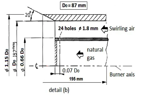
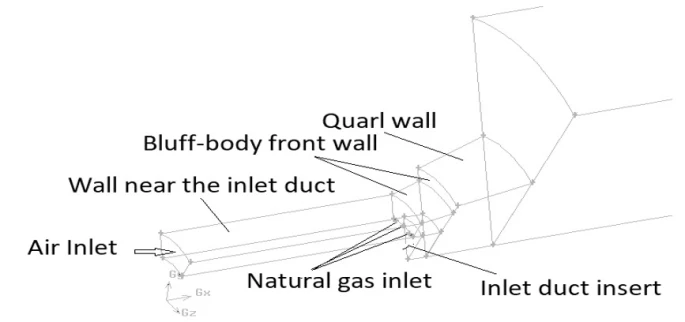
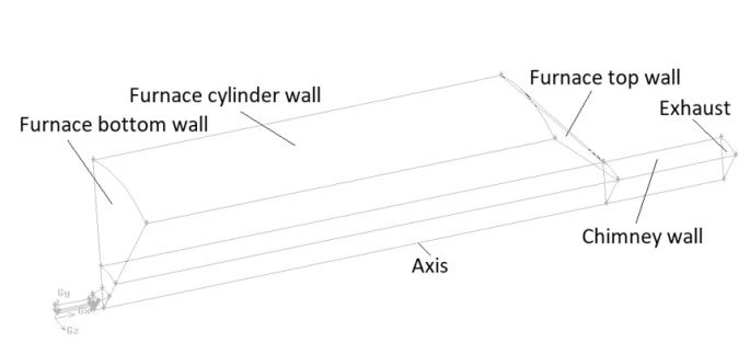
Figure 1a shows the complete geometry of the BERL combustor used in this study.      A concise description of the burner dimensions is provided in this study, and further details can be found in [2, 26]. The figure 1b also shows the longitudinal section (detailed view) of the combustion chamber. The burner dimensions were based on the outer diameter of the combustion air duct (Do = 87 mm). The injector was equipped with 24 radial gas holes, each with a diameter of Dholes = 1.8 mm. The fuel was supplied through the longitudinal tube. The operating conditions were as follows: Airflow quantity was 0.11832 kg/s at 312.15 K, and the fuel flow rate was 0.006 kg/s at 308.15 K. The swirled flow upstream of the burner chamber produced a swirl number of 0.56 in the air annulus. Computational domain was extended by 3 m axially and 1.0668 m radially.

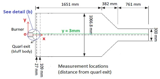
Figure 1.  a) Schematic representation of the 300 kW BERL furnace, b) Enlarged view of the burner section

a)

Full size image

b)

Full size image

Figure 2. Nomenclature of the furnace walls used for the boundary condition

a)

Full size image

b)

Full size image

Table 2. Inlet and outlet boundary conditions [2]

Full size image

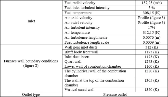
The fuel employed contains 98.4% CH4, 0.3% CO2, and 1.3% N2. The mixture of air, comprising 21% O2 and 79% N2 by mass, served as the oxidizer. Based on the fuel jet, the Reynolds number was approximately 320,000. The information used in the simulations is identical to the information used in the experiments in table 2. The diagram demonstrates the classification of the furnace walls of the BERL combustor. The labels for different wall sections were created based on their respective boundary conditions, thereby providing a clear reference for the numerical setup and ensuring consistency in the simulation framework (ANSYS FLUENT). The inlet and outlet conditions are shown in figure 3.

Figure 3. Inlet U and W velocity components [2]

Full size image

2.2. Governing equations
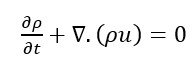
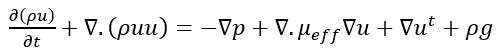
The conservative equations that represent this type of flow are

       (1)

   (2)

        (3)

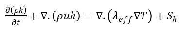
where, r is the fluid density and u are the velocity vector. h is the specific enthalpy, T is the temperature, and  is the effective thermal conductivity (laminar + turbulent). The source term Sh accounts for the contribution of chemical reactions.

      (4)

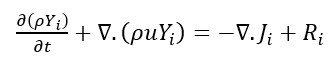
In this expression, Yi is the mass fraction of species, Ji is the diffusion flux, and Ri is the net rate of production of consumption of species i due to chemical reactions.
This equation guarantees the conservation of mass for each chemical species involved in the combustion.

   (5)

  (6)

      (7)

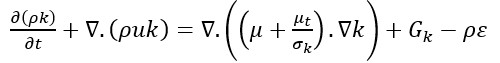
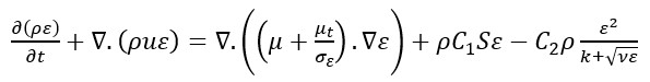
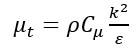
Where:  is the production of turbulent kinetic energy owing to mean gradients and   is the turbulent Prandtl number for k. With model-specific coefficients that vary with the local field. Here,  is an empirical constant that is typically set to 0.09.
Mixture fraction (f) transport equation.

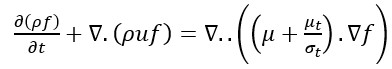  (8)

Mixture fraction variance  transport equation:

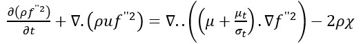  (9)

Where: st is the turbulent Schmidt number and,  is the variance of the mixture fraction fluctuations, and  is the scalar dissipation rate.

Scalar dissipation rate 

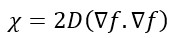   (10)

where D denotes the molecular diffusivity. The scalar dissipation rate characterizes the rate at which fluctuations in the mixture fraction are smoothed via molecular diffusion.

2.3. Numerical methods

The flow turbulent was designed using a Realizable  model with scalable wall functions so that it could be used near the wall. As for representing the radiative heat transfer, we used the model called discrete ordinates (DO) [2]. The finite volume method (FVM) is used by the Luent calculation code for the description of the differential equations of the flow and for the modeling of pressure – velocity the coupled method is used.
A second-order upwind scheme was applied for the momentum and scalar transport discretization. As for the walls of the combustion chamber, we stipulated that they must not move, meaning they must be fixed walls, and zero normal pressure gradients were applied at the boundaries. In this study, the chemical kinetics mechanism for natural gas of GRI-3.0 [28] was used.

2.4. Mesh independence study

Figure 4. a) 2D-axisymmetric mesh, b) detailed view

Full size image

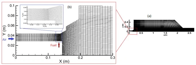
The combustion chamber mesh was generated using GAMBIT 2.2 [29] (figure 4). The mesh density was optimized to minimize numerical diffusion and ensure the stability and convergence of the simulation. Convergence was achieved when the residuals fell below 10⁻⁶. Every computation was predicated on 2D-axisymmetric configuration.
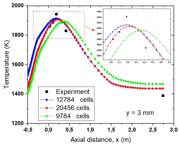
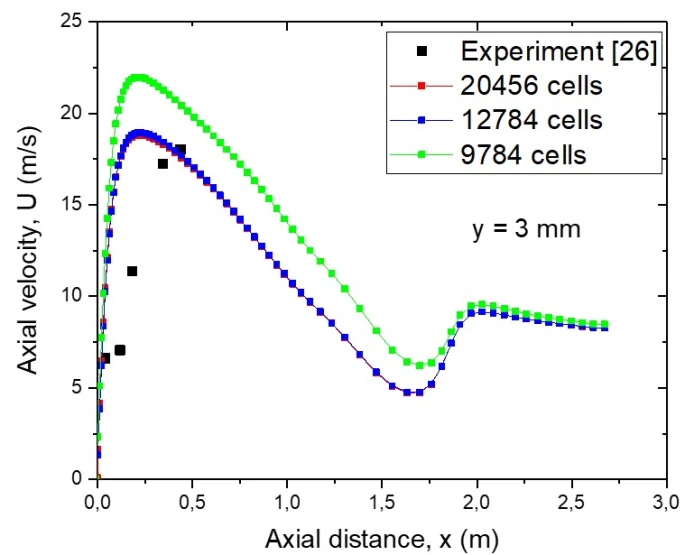
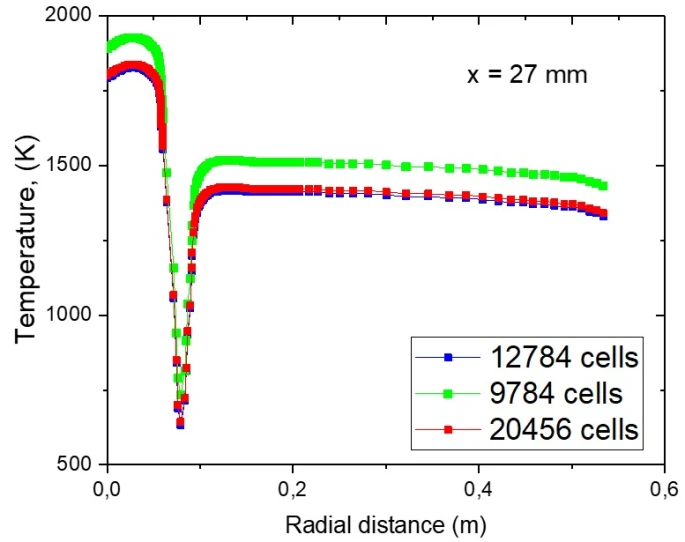
Before launching any numerical simulation calculations, it is crucial to ensure two things: the selection of a suitable mesh and the study of its independence. In our case, we selected the GRI-3.0 reaction mechanism for natural gas oxidation, and for combustion modeling, we chose the SLF model, as justified in the introduction. For this study of independence and mesh selection, we will focus on the evolution of the three most important parameters in the simulation of turbulent combustion: the flame temperature, the axial velocity, and the oxygen species. Three different types of mesh are selected for this mesh independence test: mesh 1 with 9784 cells, mesh 2 with 12784 cells, mesh 3 with 20456 cells figures 5 and 6 illustrate the evolution of the axial profiles of flame temperature and axial velocity on the line which has a distance of y = 3 mm from the axis of the combustion chamber. The temperature forecasts from every mesh displayed similar patterns, with maximum values of 1893, 1913, and 1907 K for the grid 1 (9784 cells), grid 2 (12784 cells), and grid 3 (20456 cells), respectively Nevertheless, the values ​​we obtained are in agreement and very close to the values ​​of the experimental results we used for comparison. During the experimental measuring, the maximum temperature reached 1942.55 K, with a fluctuation of less than 2.5% between grid 1 and grid 3. The grid 1 a little underestimated the results near the injector and overestimated them downstream, while the grid 2 and grid 3 provided almost identical results across the total domain. Figures 7 and 8 illustrate the radial profiles of O₂ and temperature at x = 27 mm, respectively. In general, grid 2 and grid 3 produced comparable results, thus proving that the mesh is independent of its size. Due to the reduced computational cost, a grid 2 (12,784 cells) was chosen for the following analyses.

Figure 5. Radial profiles of flame temperature at position y = 3 mm

Full size image

Figure 6. Radial profiles of axial velocity at position y = 3 mm

Full size image

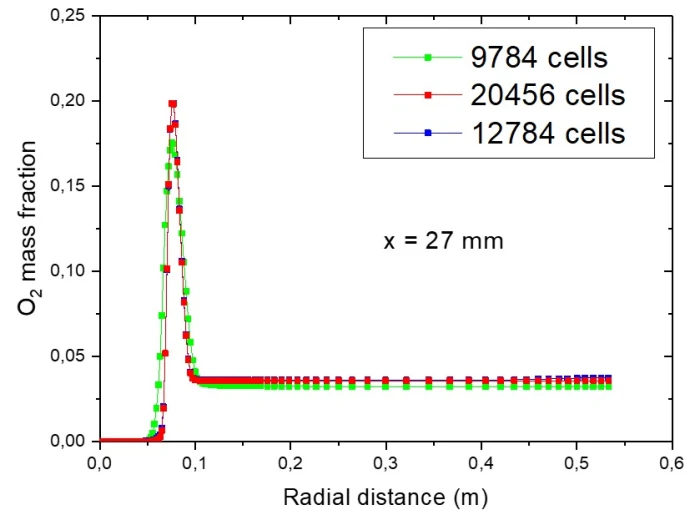
Figure 7. Radial profiles of the mass fraction of the O2 species at position x = 27 mm

Full size image

Figure 8. Radial profiles of flame temperature at position x = 27 mm

Full size image

2.5. Flamelet library for Natural gas /Air flame
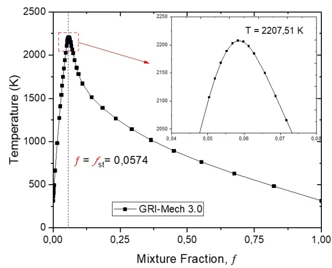
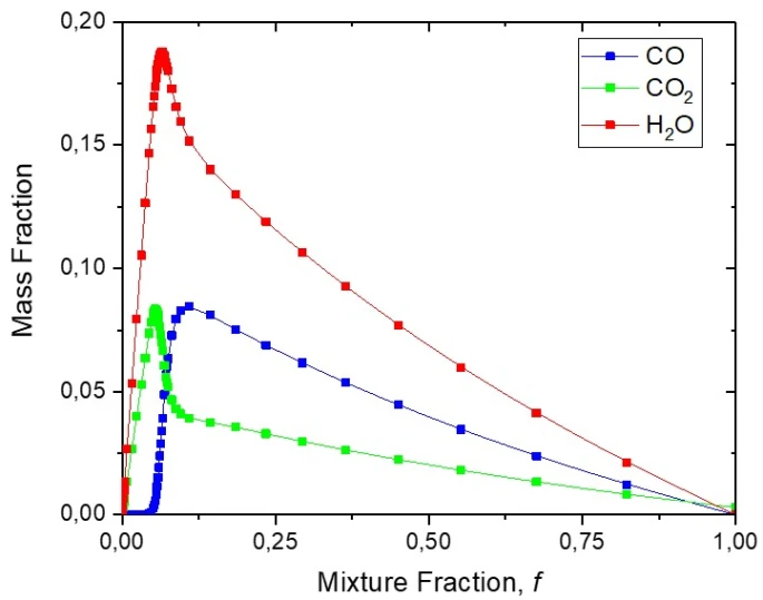
Figure 9 shows how the flame temperature varies with the scalar fraction of the mixture. The graph illustrates a rapid decrease in flame temperature, from approximately 2200 K for a scalar mixture fraction (f = 0) to approximately 300 K for a scalar mixture fraction (f = 1). This variation is characterized by the temperature distribution and pattern within a flame, where maximum temperatures are typically observed near the stoichiometric mixture fractions. A maximum flame temperature of approximately 2075.51 K was observed for a stoichiometric mixture fraction equal to fst = 0.0574. Figure 10 illustrates the radial evolution of the flamelets for the mass fractions of the chemical species CO₂, CO, and H₂O. Overall, the estimated profiles of CO₂, CO, and H₂O coincide well, thus validating the flamelet method.

Figure 9. Flamelet temperature profiles

Full size image

Figure 10. Flamelet profiles for mass fraction of CO2, CO and H2O

Full size image

Results

3.1. Temperature predictions

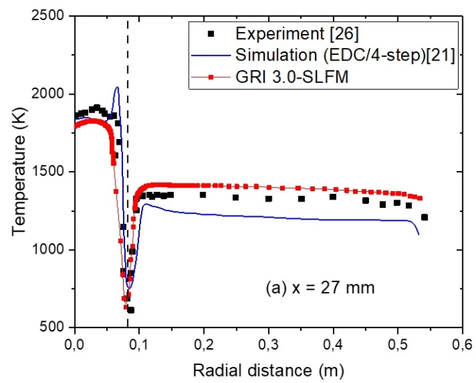
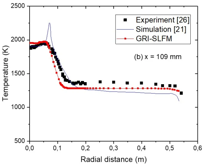
Figure 11 shows the evolution of temperatures inside the combustion chamber for two different stations taken along the chamber axis, as follows for x = 27 mm and x = 109 mm.     

At both locations along the combustion chamber axis, the results obtained using the GRI-3.0 mechanism with SLF model, there is agreement between the numerical simulations we performed and the results obtained from the experiments [26, 28], particularly in capturing the maximum temperature near the flame front and the subsequent decay in the outer radial regions. The use of the EDC combustion model with the 4-step kinetic chemistry reaction mechanism studied in reference [21] gives an underestimation of the flame temperature on the combustion chamber axis or the gradient on the flame fronts, and less estimates this tendency to continue to diverge in the far region of the flame. In the region near the injector at x = 27 mm, the SLFM combustion model correctly reproduces the temperature behavior of the flame which gives rise to a stable zone for the flame. In the region furthest from the injector outlet at x = 109 mm, the continuous SLFM combustion model accurately represented the temperature distribution calculated numerically and obtained experimentally. The SLFM model, coupled with the detailed mechanism of GRI-3.0, captured the temperature peak in this region. These results prove the power of the SLFM model for the qualitative and quantitative representation of flame structure behavior. We have drawn up a table 3 which compares the maximum flame temperatures for the measurement station along the axis of the flame, that of x = 27 mm and that of x = 109 mm, with those obtained experimentally cited in reference [26], and at the same time we use another numerical study cited in reference [21] for the validation of our work. The work cited in reference [21] using EDC as a model for combustion modeling with an overall four-stage process. The EDC model's predictions were farther from the experimental measurements than the SLFM predictions at both positions. The EDC model overestimated the temperature by 2047 K vs. 1910.73 K at 27 mm, while the present work slightly underestimated it (18878.5 K), which was within a reasonable deviation. The SLFM prediction (1973.77 K) was much more accurate for x = 109 mm than the EDC result (2252.53 K), which overestimated the flame temperature significantly. It has been confirmed that the utilization of GRI-Mech 3.0 in the SLFM framework enhances the predictive accuracy by capturing both near-field and far-field flame temperatures with a lesser error compared to experimental benchmarks.

Figure 11. Temperature profiles at two locations, at x = 27 mm and at x = 109 mm

a)

Full size image

b)

Full size image

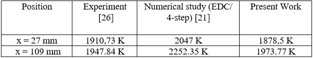
Table 3. Examining the maximum flame temperatures at two locations: at x = 27 mm and x = 109 mm

Full size image

3.2. Velocity profiles
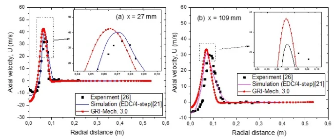
The axial velocity evolution at different positions along the combustion chamber axis is shown in figure 12, where it is compared with experimental results. In general, these results show better agreement between the two. For the measurement station (x = 27 mm), the opposing velocities defined in the internal recirculation zone were higher than those measured experimentally. Subsequently, the simulation showed a negative velocity of approximately -17 m/s on the central axis of the combustion chamber, while experimental measurements showed only -8 m/s as the velocity value at the same positions. This difference between the two values ​​may be due to the first-order turbulence model's inability to accurately determine the anisotropy and dissipation in this region, which is dominated by strong vortex recirculations linked to highly turbulent flow.
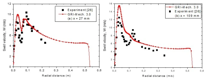
This discrepancy can be attributed to the limited capability of the turbulence model to represent anisotropy and dissipation in the highly turbulent recirculation region. In contrast, the simulation with the GRI-Mech 3.0 mechanism produced peak values that were in closer agreement with the experimental data at both measurement stations. In general, the axial velocity field was well captured, particularly near the nozzle. The swirl velocity components are depicted in figure 13, where the results predicted through simulation are in good agreement with the experimental, up to y = 0.1 m, but show increasing deviations both qualitatively and quantitatively further downstream.

Figure 12. Radial profiles of axial velocity, U (m/s): a) x = 27 mm, b) = 109 mm

Full size image

Figure 13. Radial profiles of swirl velocity W (m/s): a) x = 27 mm, b) x = 109 mm

Full size image

3.3. Radial profiles of mass fractions of O2 and CO2
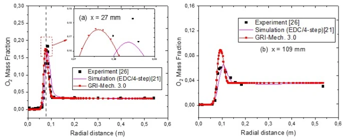
Figure 14 shows the radial distributions of the O₂ mass fraction. At x = 27 mm, the predictions using the GRI-Mech 3.0 mechanism reproduced a peak value of the O₂ mass fraction, which was in good concordance with the experimental data (figure 14a). At x = 109 mm, the detailed mechanism yielded slightly lower peak values, which improved consistency with the experimental results. Overall, the predicted profiles showed good agreement with the measurements, although oxygen burnout was under-predicted at the first station. This underestimation corresponded to a lower predicted CO₂ mole fraction at the same location. From figure 14, it can be observed that the detailed mechanism provided only marginal improvements in predicting the O₂ radial distributions at x = 109 and 343 mm. Figure 15 shows the CO₂ mass fraction distribution curve. The profiles obtained using the GRI-Mech 3.0 mechanism agreed reasonably well by means of the experimental data, except for a slight radial shift toward the burner. Although both models adequately predicted fuel consumption, neither captured CO₂ formation with high accuracy.
In particular, the flame model tended to overestimate both the peak values and O₂ and CO₂ mass fractions along the flame axis. This behavior is consistent with the overestimation of the differential diffusion effects incorporated in the flamelet library, which accounts for the observed discrepancies.

Figure 14.  Radial profiles of O2 mass fraction: (a) at x= 27 mm, (b) x = 109 mm

Full size image

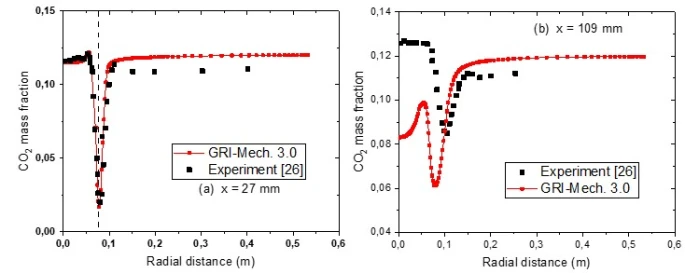
Figure 15.  Radial profiles of the mass fraction of CO2 (a) at x= 27 mm, (b) x = 109 mm

Full size image

3.4. Effect of H2O addition to the fuel and air
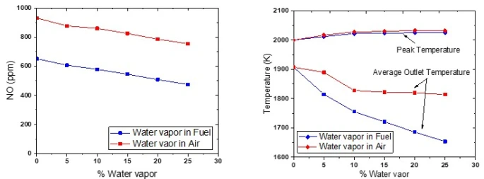
This study investigated the effect of water vapor addition on the combustion characteristics, such as temperature and emissions (CO₂, CO, and NO), of a swirl-stabilized natural gas burner. All other fuel and air jet parameters were kept constant, as shown in table 2. The water vapor mass fraction was varied in increments of 5% from 0% to 25%. Data analysis indicated that when water vapor was incorporated into the fuel at a mass fraction of 25%, water contributed approximately 2% of the total mass of the mixture. Moreover, the overall mass flow rate through the burner increased with the addition of water vapor to the fuel. In the context of this study, 12 simulations were performed to evaluate the effect of adding water vapor to the combustion chamber. Generally, emissions produced by natural gas combustion are primarily composed of nitrogen oxides (NOx), carbon monoxide (CO), carbon dioxide (CO2), and other minor pollutants. Figure 16 shows the distribution of NO as a function of the percentage of water vapor contained in methane and in air. Ultimately, there are 12 cases to study using numerical simulation. In both graphs, we note that the amount of NO released during combustion decreases as the amount of water vapor ejected increases, either into the methane or the air. We can observe that injecting water vapor into the methane results in a lower amount of NO and a rapid decrease compared to injecting it into the air. Figure 16b illustrates the evolution of flame temperature as a function of the percentage of water vapor added to both sides (methane and air). It is clear that the temperature at the combustion chamber outlet decreases rapidly compared to the temperature at which water vapor is injected into the air; a statistical comparison can be made for each case.
The behavior of the evolution of the CO mass fraction is illustrated in figure 17 for the two simulation cases. It is noted that a value of 14 times less CO than the flame containing no water vapor, i.e., 0% water vapor in the methane. Figure 18 a clearly shows the effect of adding water vapor to methane on the distribution of the CO₂ mass fraction. As the amount of injected water vapor increases from 0% to 25%, the CO₂ concentration drops from 0.1295 to 0.1088. Consequently, dilution of the air by water vapor results in a nearly constant variation (figure 18 b). There is a clear difference between 0.1292 and 0.1294 indicating that there is no correlation between the percentage of water vapor added to either natural gas or air.

Figure 16. (a) NO produced, (b) distribution peak, and average outlet temperature

Full size image

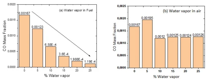
Figure 17.  Mass fraction of CO (a) for vaporized water in fuel; (b) for vaporized water in air

Full size image

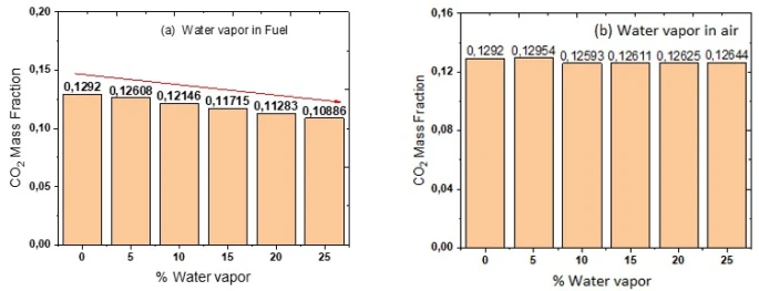
Figure 18. Mass fraction of CO2: a) for vaporized water in fuel, b) for vaporized water in air

Full size image

Figure 19 presents the static temperature contours (K) in the combustion chamber for water vapor mass fractions ranging from 5% to 25%, comparing steam injection into the fuel and into the air. Increasing the water vapor content modifies the thermal field and slightly reduces the high-temperature regions. This behavior is mainly due to dilution effects and the reduction of the adiabatic flame temperature. Steam injection into the fuel has a more pronounced impact on the thermal structure than injection into the air. In addition, the flame length in the recirculation zone decreases, as indicated by the black line in figure 19.

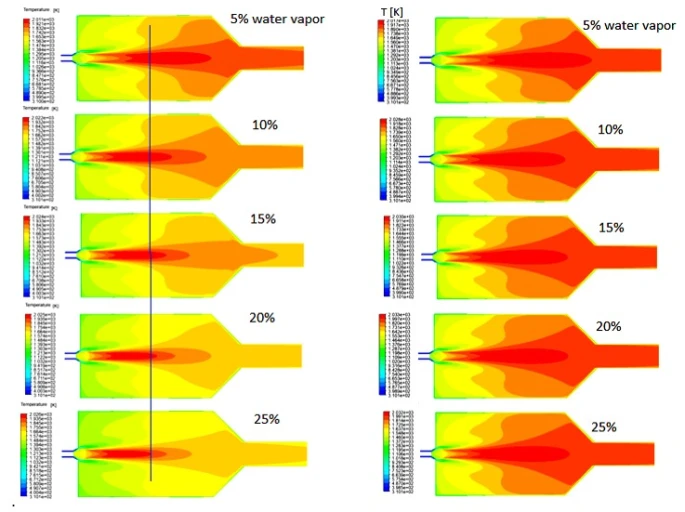
Figure 19. Contours of static temperature (K): Vapor water added to the fuel. (b) Vapor water is added to the air

Full size image

Conclusion

This study evaluated the application of the Steady Laminar Flamelet Model (SLFM) coupled with the detailed GRI-Mech 3.0 mechanism for modeling non-premixed turbulent combustion in a swirl-stabilized natural gas burner. The simulation results show a perfect correlation with experimental data, especially for the radial evolution of axial and tangential velocities along the combustion chamber axis, and the same for the mass fractions of chemical species such as NO and carbon dioxide. However, there is some difference between the results of the simulations and the experimental measurements in the area of ​​strong gradient i.e. in the recirculation zone, where we note that the evolution of carbon dioxide gives curves quite concordant with this experimental data, these differences may be linked to the turbulence model itself i.e. the anisotropy of the turbulence and to the effects of molecular diffusion. Based on these results, it became clear to us that adding water vapor to natural gas has a significant impact on the combustion system and the toxic substances produced. Diluting the natural gas in our case, purely methane has a remarkable effect on reducing nitrogen oxides (NOx) because the flame temperature at the center of the combustion chamber has decreased. Dilution of the air by adding water droplets to the spray resulted in a very high flame temperature and, simultaneously, a reduction in NO pollutant emissions. In conclusion, this work demonstrates that the SLFM combustion model is well-suited and effective for studying reactive turbulent flows such as flame diffusion, coupled with a detailed kinetic chemistry model like GRI 3.0. This study contributes to the strategy for removing polluting chemical species from combustion chambers in gas turbines, and this technique appears to be a promising method. Future studies should focus on improving the modeling by using second-order turbulence models such as RSM.

References

About this article