UNEC Journal of Engineering and Applied Sciences Volume 5, No 2, pages 45-57 (2025) Cite this article, ![]() 2562 https://doi.org/10.61640/ujeas.2025.1204
2562 https://doi.org/10.61640/ujeas.2025.1204
Micron- and submicron-sized particles used in industry and technology have magnetic properties (dia or paramagnetic) in many cases. Therefore, significant research has been conducted on the application of high gradient magnetic fields for the separation of such magnetic particles in many fields including medicine, biology and bioengineering [1,2]. Among these application areas, minerals benefication [3,4], drug and gene delivery [5,6], manipulation and control of cells [7,8], magnetic resonance imaging [9] and hyperthermia [10], are more prominent. In generally, high gradient magnetic separators (HGMS) are widely used for the separation of micron-sized particles [11]. The principle of transport or retention of magnetic nanoparticles is based on the magnetophoresis processes [12-15]. Widely, the powerful permanent magnets (especially of the (NdFeB) type) or electromagnetic coils are used as the external magnetizing system [16]. However, as particle sizes decrease, conventional magnetic separators are insufficient for the separation of submicron particles [2,4]. In many cases, especially in medical and biological systems, the magnetic separators used in separation processes should be smaller and miniaturized [17-19]. In this case, it is impossible to use the conventional magnetization system coils used in magnetic separators. Therefore, permanent magnets are mainly used as external magnetization source in these systems [19]. In this context, The performance of the magnetophoresis processes, depends mainly on the value of the magnetic field generated in the separation zone [4,20]. Recently, magnetophoresis processes have been widely applied in microfluidic systems [21,22]. In such systems, the focusing of magnetic particles remains as a major problem [23-28]. Because it is important to obtain the position coordinate of the maximum values of the magnetic field gradient of the magnetic separators in these cases. The magnetic fields generated by permanent magnets for separation zone in magnetophoresis systems are relatively weak and cannot be adjusted [29]. Therefore, obtaining large values of the magnetic field in the separation zone is only possible by choosing a suitable geometry for the magnetic system [30]. Generally, in microfluidic magnetophoresis systems, mainly rectangular or disk-shaped magnets are preferred to match the geometry of the separation channel [20]. The investigation of magnetic fields generated by different types of magnets has been well reviewed in the literature [29]. Nevertheless, the all-around treatment of magnetic fields generated in different ways in accordance with the geometry of the separation channel has still not been sufficiently investigated. In particular, simple models that can be easily used in engineering calculations of the gradient magnetic field of different configurations are few and inadequate, as well. This is because the analytical formulas derived from the magnetic potential theory approach [31]. This traditional approach to the determination of such magnetic fields, are complex and not very convenient for practical calculations. Accordingly, the problem of obtaining analytical or approximate analytical formulas that are more useful for engineering calculations in this field remains important [20,32,33]. On the other hand, the limited size of permanent magnets and the weakness magnetic field that generate make this problem difficult to solve. Therefore, to obtain high gradient magnetic fields in microfluidic channels, it is necessary to combine a permanent magnet and ferromagnetic elements (ball, wire, prism, etc.) magnetized by the effect of this magnet [34-37]. In this case, the magnetic field gradient in the separation channel is high the magnetic force acting on the microparticles in this area is increased. The calculation of such fields are required special approaches that different from the magnetic potential theory solutions [38].
In this paper, the variation of the gradient magnetic field generated by magnetized ferromagnetic balls under the influence of permanent magnets is investigated. Using the approximate approach, the general expression of the magnetic field in the separation zone is established. This empirical formula is obtained taking into account the magnetic and geometrical properties of the magnetization system. Measurements were performed between ferromagnetic balls of different sizes and quantities (above the separation channel) using neodymium (NdFeB) magnets. The accuracy of the derived approximate analytical formula is tested by experimental results. The obtain results show that the theoretical and experimental results are in good compatibility.
Write For the measurement of the non-homogeneous magnetic field generated by magnetized ferromagnetic balls, it has preferred to use a magnetometer operating on the Hall probe principle [37]. For this purpose, a specially designed Hall probe portative magnetometer working on the principle of 3D printer is used [38].
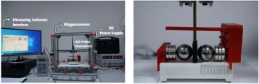
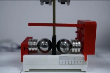
The general appearance of this 3D principal magnetometer is shown in figure 1a. It has an operating platform made mainly of non-magnetic materials which can be moved up and down independently. Also has a moving mechanism with a Hall probe mounted on the magnetometer. With three stepper motors placed on the carrier structure, these parts can be moved in 𝛿 ≤ 0.1mm steps, allowing precise measurement of magnetic field intensity in three dimensions (x,y,z). The step values of the Hall probe can be realized manually or automatically by computer. The non-homogeneous magnetic field is generated in a specially designed measuring cell (figure 1b).
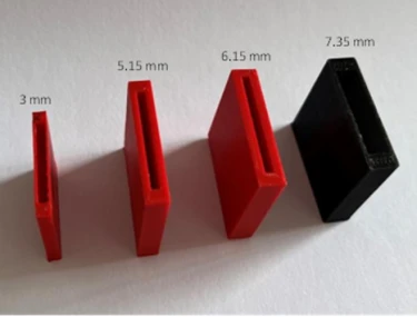
NbFeB magnets with a diameter of 50 𝑚𝑚 and a thickness of 𝑙𝑚 = 10 𝑚𝑚 were used as the magnetic field source. The positions of the side walls of the measuring cell, which is placed on the platform of the magnetometer, are designed to be adjustable. Thus, it is possible to create magnetic fields with different magnetic field intensities by changing the distance between the magnets. High gradient magnetic fields are obtained by placing ferromagnetic balls between NdFeB magnets and in the spaces between these balls.
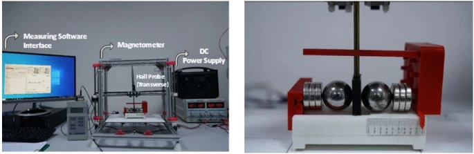
Figure 1. a) measuring setup for magnetic field, b) magnetometer with transverse hall probe – measuring cell
a) b)
High gradient magnetic fields between ferromagnetic balls were measured with Hall probe gaussmeters. Ferromagnetic balls used 100Cr6 label with diameters of 2𝑎 = 33.35 mm, 16 mm, 15 mm and 6 mm were used in the experiments In order to avoid touching between magnetized balls and to measure the magnetic field in these regions with Hall probes, special channels with air gap were designed in 3D printers. These channels are made of hard plastic materials which are hollow inside (figure 1c). In order to evaluate the constructive measurement errors of the portable magnetometer, both the G05 Gaussmeter and the LakeShore Model 410 Gaussmeter and their Hall probes were used in the same measurements. Depending on their location, measurements were performed using both axial and transversal Hall probes. The data of both measuring instruments were practically equivalent. The measurement results of the G05 Gaussmeter were taken as reference for the final data. More than a thousand measurements were performed in the experiments and the data obtained were statistically analyzed.
2.2 Theoretical Analysis
In generally, the investigation of the magnetization properties of magnetic materials with different geometries in external homogeneous and inhomogeneous magnetic fields are one of the most important and classical problems of electromagnetic field theory.
However, magnetized magnetic materials with special structures are used in many emerging technologies and nanotechnologies. The study of the magnetic fields of these materials, especially wire, rod and spherical elements, in different situations remains a contemporary problem. Because in this case it is possible to generate effective magnetic fields with high gradients in miniaturized magnetic systems [4,20,34]. On the other hand, magnetization systems have limited magnetic field intensity. Therefore, obtaining a high magnetic field gradient in the study region was determined as the main objective in similar studies [20].
The classical approach that followed to calculating the magnetic field around magnetized elements (balls, wires etc.) in an external magnetic field uses the definition of static field potential [4]. However, by using this approach, the calculation of the gradient fields around balls and wires in the external field created by permanent magnets is obtained by complex analytical formulas [20,31] . In particular, this method is insufficient for the determination of magnetic fields around magnetized and tangent magnetic elements [21,39,40]. Because it is not straightforward to determine the potential distribution when magnetized ferromagnetic elements are touching to each other. Whereas, ferromagnetic elements used in microfluidic magnetophoresis systems are often tangent to each other Accordingly, the use of some approximate methods in the calculation of gradient fields around magnetized ferromagnetic balls and wires allows simpler results to be obtained in terms of practical calculations [4,21,38-42].
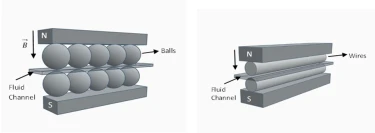
Approximate analytical formulas proposed by many researchers for the determination of the magnetic field in packed beds formed by a large number of ferromagnetic balls magnetized in an external magnetic field have been presented in the literature [40,43,44]. However, the determination of the approximate analytical expression of the gradient magnetic field generated by a limited number (one, two, three) of balls magnetized with permanent magnets requires consideration of some different properties. Since, these systems have serious criteria in terms of both the strength of the magnetic system and the geometry and size of the entire system. For this reason, the analysis of magnetophoresis phenomena in microfluidic systems is nowadays considered in terms of these criteria. Typically, the easiest approach to increase the magnetic field gradient in flow channels in microfluidic systems is to change the pole geometry of the external permanent magnets [4,20]. However, in some cases, this approach may not be advantageous depending on the application of microfluidic magnetophoresis. Therefore, in microfluidic magnetophoresis systems, placing a small ferromagnetic ball or wire between the permanent magnet and the channel to generate a high gradient magnetic field can be used as an effective method [37]. The principle schematics of similar systems are shown in figure 2. The fact that the gradient magnetic field generated in these systems decreases rapidly away from the surfaces or tangent points of the magnetized ferromagnetic ball or wire can be used as a determining factor of the variation of these fields [39-44]. This factor can be taken into account for theoretical investigations as a sufficient condition for establishing approximate analytical formulas of gradient magnetic field variation in these systems [38].
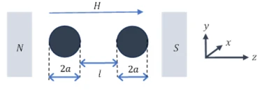
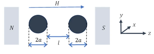
In this study, the analysis of gradient field generated between ferromagnetic balls magnetized by using permanent magnets is considered. The principal schematic of two small-sized ferromagnetic balls with radius 𝑎 and distance 𝑙 between them, magnetized by the effect of an external permanent magnet, is shown in figure 3.

Figure 2. Principal schematic for gradient magnetic field in channel. a) with magnetized ferromagnetic balls, b) with magnetized ferromagnetic wires
a) b)
It is obvious that in such systems demagnetization events are more effective. Because of that the analytical formulas obtained in terms of static magnetic potential are mathematically quite complicated [43,44]. For this reason, some studies have used different approximate methods to calculate the magnetic fields in such systems [30,38,39,42]. In these studies, for example in reference [39] finite analytical results are obtained using a simple approximately approach. As such, it has been shown by numerous experimental studies in reference [39] that the magnetic field variation between magnetized balls or wires is similar. It can be determined by the following general expression.
 (1)
(1)
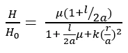
Here,  and
and  are correction coefficients that depend on the properties of the magnetization system and determining from experiments, 𝑎 is the radius of the ball, 𝑦 is the distance between the balls from the center (
 ),
),  is the external magnetic field strength.
Generally, in a chain of magnetized balls, the magnetic field lines are concentrated around the tangent points of the balls or parallel to the axis of symmetry [21,39]. Therefore, the radial coordinate 𝑟 in cylindrical coordinates can be written instead of the usual 𝑦 in equation 1. In this study, using the average magnetic permeability definition of permanent magnets in magnetic media [34], equation 1 is obtained as follows.
 (2)
(2)
Here,  is the relative magnetic permeability of the balls, l is the gap between the balls,
 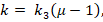 is the coefficient that depends on the geometrical and magnetic properties of the magnetization system,
  is the correction coefficient.
In experiment, the variations of the induction gradient magnetic fields from limited number and different diameters of ferromagnetic balls were measured with precision. The compatibility of the obtained results with equation 2 is evaluated.
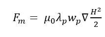
Considering equation 2, the magnetic force acting on micron and submicron particles in the channel placed between ferromagnetic balls is determined as follows.
 (3)
(3)
As seen from equation 3, the amplitude of the magnetic force acting on particles in magnetophoresis events is directly proportional to the factor  . Considering equation 2, it is also obvious that this factor has an extremum region. This result emphasizes the advantage of using a gradient magnetic field in magnetophoresis processes.
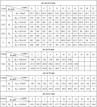
The measurement of the variation of the gradient magnetic field in the separation channel between magnetized ferromagnetic balls under the influence of permanent magnets was carried out in the prototype magnetometer, measuring cell shown in figure 1. The step change of the sensitivity of the Hall probe in the measurements is 0.1 mm. In the experiments, the variation of the basis magnetic field intensity ( ) was obtained by varying the number of magnetizing NbFeB magnets. The effect of increasing the limited number of magnetized balls in chain on the variation of the magnetic field in the channel was also studied. In all cases, first of all the basis magnetic field intensity (
 ) was measured for the case where without ferromagnetic balls between the magnets. Considering that the magnetization of the ferromagnetic balls is symmetric, the measurements were made from the center of the channel between the balls along the 𝑦 -axis (figure 3). In order to evaluate the magnetization effect of the magnetic balls, measurements were made starting from the symmetry axis of the balls (y = 0) towards higher points (y >0). The obtained results are discussed in tables and graphs. Table 1 shows all the measurement results for different channel width (𝑙) by using one and two neodymium magnets.
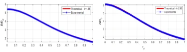
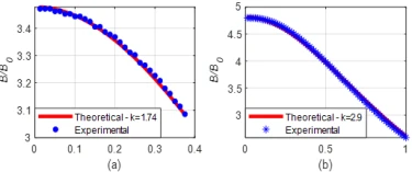
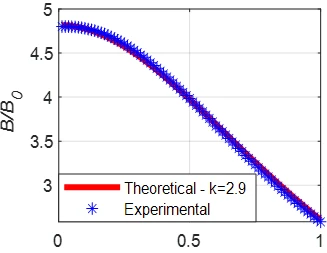
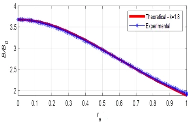
As can be seen from table 1, the basis magnetic field intensity ( ) in the measurement region increases with increasing number of magnets. On the other hand, it is obviously seen that the increase in magnetic field intensity is higher when ferromagnetic balls are placed in the test region. Figure 4 shows the magnetic field variation for 2a = 33.35 mm balls using 2 and 4 neodymium magnets in the case of l =7.35 mm channels. As seen in figure 4, the magnetic field between the balls increases rapidly as the channel width l decreases. As expected, the highest value of the magnetic field is on the center axis between the balls in all cases. On the other hand, when the coefficient 𝑘 shown in equation 2 is adjusted, the theoretical and experimental results of magnetic field variations in different structures coincide. Moreover, these results depend on the magnetic permeability 𝜇 of the balls and are similar to the variation characteristics of 𝜇. In other words, unlike the magnetic field generated by the case without balls, the maximum point of the magnetic field gradient in the channel occurs when ferromagnetic balls are placed in this region. This allows to determine the focusing point of the maximum magnetic force zone in the channel. Therefore, in this case it is possible to obtain the best performance of the magnetophoresis process.
Table 1. The measurement results for different channel width (𝑙) by using one and two neodymium magnets

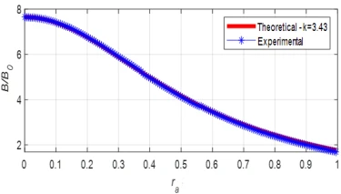
Figure 4. Variation of  with
with  for magnetized ball with
  mm, l =7.35mm. a) for a pair of magnets, b) for two pairs of magnets
a) b)
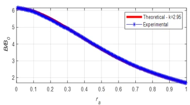
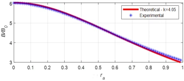
Similar results to those obtained for l = 7.35 mm were obtained for other different channel widths (figures 5-6-7). In all calculations the coefficient  in equation 2 has been corrected for each case. The important feature here is that
  in all cases. This is due to the dependence of the coefficient
  on the demagnetization properties of the magnetization system.

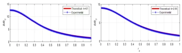
Figure 5. Variation of  with ra for magnetized ball with
  mm, l =6.15 mm. a) for a pair of magnets, b) for two pairs of magnets
a) b)

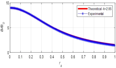
Figure 6. Variation of  with ra for magnetized ball with
  mm, l =5.15mm. a) for a pair of magnets, b) for two pairs of magnets
a) b)
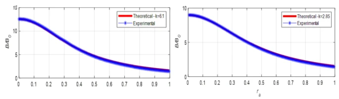
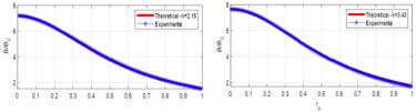
Figure 7. Variation of  with ra for magnetized ball with
  mm,
mm,  mm. a) for a pair of magnet, b) for two pairs of magnets
a) b)
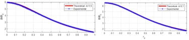
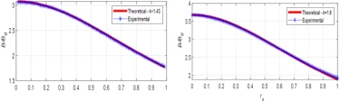
Figure 8 shows the experimental and theoretical results obtained similar to the above measurements for the case where the  mm between the 2a= 16mm ferromagnetic balls. Figure 8a shows the magnetic field variation in the channel between the two balls are used. Figure 8b and 8c show similar results for four balls and six balls respectively. In general, the change characteristic of the magnetic field is similar in the all cases. However, with the increase in the number of balls in the magnetization chain, the magnetic field increase is higher due to the decrease in the demagnetization properties (table 1). On the other hand, the advantage of increasing the magnetic field in the channels is a disadvantage in terms of dimensions for magnetophoresis processes. In order to keep the dimensions of the magnetic systems small in such structures, both the dimensions and the number of balls must be limited. In this case, it is more convenient to make the chain of magnetized balls in the longitudinal direction rather than in the transverse direction of the fluid channel (figure 2a).
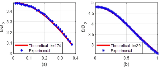
Figure 8. Variation of  with ra for magnetized ball with
  mm, l=7.35mm. a) for one ball for each side, , b) for two balls for each side
a) b)

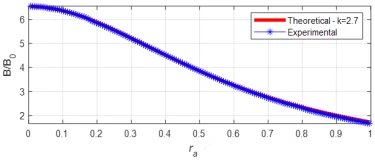
Figure 9. Variation of  with
with  for magnetized ball with 2𝑎 = 15 mm,
  mm. a) for one ball for each side, b) for two balls for each side
a) b)
Figure 9 shows the experimental results for  mm balls with an inter-sphere channel width l=7.35 mm. As seen in figure 9, the magnetic field variation in this case is in compliance with the variation in figure 8. When all these findings are evaluated, it can be concluded that although the diameter of the magnetized balls varies over a wide range of
 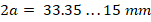 , the magnetic field variation in the inter sphere channel shows the similar characteristic. That is, in all cases, the magnetic field decreases rapidly away from the inter sphere center and the magnetic field gradient has a region of maximum. On the other hand, as the diameter of the magnetized ferromagnetic balls decreases, the maximum value of the magnetic field also decreases. However, as expected, the magnetic field values become higher as the distance between the balls decreases. When the ferromagnetic balls are tangent (𝑙 = 0), the generation of the gradient magnetic field can reach the highest values around the tangent points. In this case, the saturation of the magnetic field intensity near the tangent points of the magnetized balls is also observed [21].
The saturation level of the generated magnetic field is reached around basically at 𝑟/𝑎 ≤ 0.1 … 0.17 [21,39]. At high values of strong external magnetic fields (electromagnetic coils), the balls are more likely to reach saturation values around the tangent points. However, in magnetophoresis processes in microfluidic systems, this saturation phenomenon is unlikely to occur in ferromagnetic balls separated by flow channels. As can be seen from equation 2, one of the main parameters affecting the magnetic field variation in the microfluidic channel between ferromagnetic balls is the  coefficient. As mentioned above, the main factor determining the
  coefficient is
  , the magnetic permeability of the ferromagnetic balls. Ferromagnetic balls used in magnetic separation and filtration processes usually have highly 𝜇 [21].
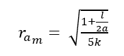
The magnetic field strengths generated in microfluidic channels by NbFeB magnets used in magnetophoresis processes are  < 150 − 200 kA/m. Considering these results, the position where the magnetic force acting on the particle in the fluid channels is maximum can be easily determined according to equation 4.
 (4)
(4)
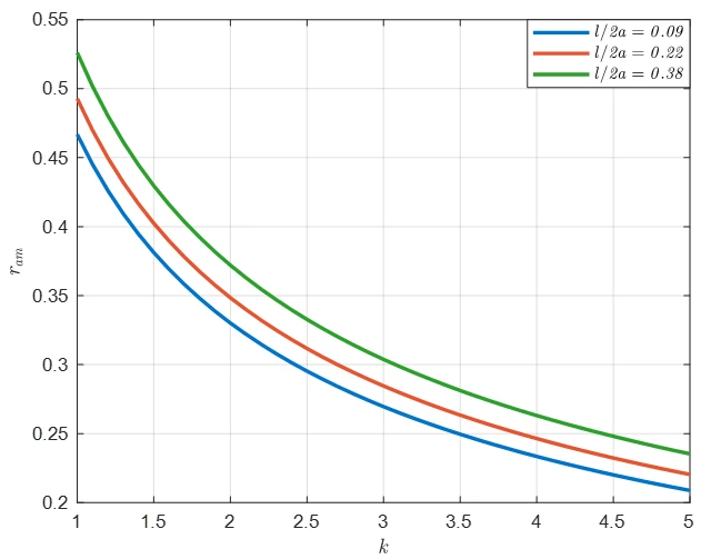
Figure 10 shows the variation of the position where the magnetic field is maximum ( ) with respect to
  in equation 4 for different values of
  .
.
As can be seen from figure 10,  decreases rapidly with increasing
  and hence
  , for all cases of
  . Therefore,
  must be taken into account in determining the regions where the magnetic force is maximum. This result is important in the design and theoretical calculation of magnetophoresis systems. Similar results were obtained in the studies presented in the literature for HGMSs with ferromagnetic packed beds [21,39].
As mentioned above, in all these gradient field cases, the magnetic field gradient or magnetic force  in equation 3 has a maximum value with respect to the
  . Therefore, we can easily determine the location zone of the maximum force with respect to the radial coordinate r via equation 3.
As can be seen from equation 4,  decreases in weak magnetic fields (for large 𝜇 values) created by permanent magnets. Therefore, in magnetophoresis processes in microfluidic systems, it is possible to tune the region where the magnetic force acting on the particles in the channels placed between the ferromagnetic balls is maximum.
In microfluidic magnetophoresis processes, it is necessary to increase the magnetic field gradient in the separation channels in small size magnetic systems using permanent magnets. For this purpose, it is more advantageous to use magnetized ferromagnetic elements (balls or wires) together with these magnets. Because the use of magnetized ferromagnetic elements allows the formation of a magnetic field with a higher gradient at local points of the flow channel of the system. Experimental investigations have shown that the variation characteristics of the magnetic field in the channels are approximately similar when large or small diameter ferromagnetic balls are used as structural models. This similarity is also obtained when the number of magnetized balls is varied. In order to generate magnetic fields in magnetophoresis channels, a homogeneous magnetic field is created mainly by using rectangular permanent magnets. Since the values of this magnetic field in the channel cross-section are limited, the force effect on the magnetic particles in this region is also limited. However, when the magnets are used tangentially with ferromagnetic elements, the magnetic force acting on the particles increases effectively due to the magnetic field gradient. This force also creates a gradient magnetic field region with a maximum value in the channel. This result can be used as an advantage for more efficient focusing of submicron magnetic particles in fluid channels or to improve the performance of the system. In such systems, an approximate analytical formula for the magnetic field generated between ferromagnetic elements can be derived from the general characteristics of the magnetization system. These magnetization characteristics can be determined according to the continuous increase or decrease of the magnetic field, boundary and initial condition values. In this study, the approximate analytical formula (equation 2) obtained by this method coincides with the experimental results. Accordingly, the proposed approximate analytical expression can be used in the analytical investigation of the motion dynamics of particles held or focused in microfluidic magnetophoresis. On the other hand, the approximate analytical expression for the magnetic field generated by ferromagnetic balls tangent to each other is also obtained when 𝑙 = 0 in equation 2. This result can be applied to the design study and modeling of packed beds, which are widely used in high gradient magnetic separation and filtration systems.
1 C. Alexiou et al., IEEE Transactions on Applied Superconductivity 16(2) (2006) 1527. https://doi.org/10.1109/TASC.2005.864457
2 K.E. McCloskey, J.J. Chalmers, M. Zborowski, Analytical Chemistry 75(24) (2003) 6868. https://doi.org/10.1021/ac034315j
3 J. Strayer et al., Separation and Purification Technology 368 (2025) 132994. https://doi.org/10.1016/j.seppur.2025.132994
4 J. Svoboda, Magnetic Techniques for the Treatment of Materials, Springer (2004). https://doi.org/10.1007/1-4020-2107-0
5 M. Tesanovic, J.P. de Souza, M.Z. Bazant, S. Berensmeier, AIChE Journal (2025). https://doi.org/10.1002/AIC.18733
6 J. Dobson, Nanomedicine 1(1) (2006) 31. https://doi.org/10.2217/17435889.1.1.31
7 B.D. Matthews, D.A. Lavan, D.R. Overby, J. Karavitis, D.E. Ingber, Applied Physics Letters 85(14) (2004) 2968. https://doi.org/10.1063/1.1802383
8 I. Šafařík, M. Šafaříková, Journal of Chromatography B 722(1–2) (1999) 33. https://doi.org/10.1016/S0378-4347(98)00338-7
9 C. Sun, J.S.H. Lee, M. Zhang, Advanced Drug Delivery Reviews 60(11) (2008) 1252. https://doi.org/10.1016/j.addr.2008.03.018
10 B. Thiesen, A. Jordan, International Journal of Hyperthermia 24(6) (2008) 467. https://doi.org/10.1080/02656730802104757
11 X. Zheng, Z. Xue, Y. Wang, G. Zhu, D. Lu, X. Li, Powder Technology 352 (2019) 159. https://doi.org/10.1016/j.powtec.2019.04.048
12 M.M. Tagiyev, K.F. Aliyeva, UNEC Journal of Engineering and Applied Sciences 5(1) (2025) 70. https://doi.org/10.61640/UJEAS.2025.0508
13 U.N. Naghiyeva, S.R. Hajiyeva, F.V. Hajiyeva, UNEC Journal of Engineering and Applied Sciences 5(1) (2025) 83. https://doi.org/10.61640/UJEAS.2025.0509
14 M.G. Toudeshkchouei, H. Abdoos, Biomedical Microdevices 26(1) (2024) 1. https://doi.org/10.1007/S10544-023-00693-9
15 P. Noosawat et al., Microfluidics and Nanofluidics 26(10) (2022) 1. https://doi.org/10.1007/S10404-022-02583-7
16 Y. Moser, T. Lehnert, M.A.M. Gijs, Applied Physics Letters 94(2) (2009). https://doi.org/10.1063/1.3072592
17 L.E. Udrea, N.J.C. Strachan, V. Bǎdescu, O. Rotariu, Physics in Medicine & Biology 51(19) (2006) 4869. https://doi.org/10.1088/0031-9155/51/19/010
18 Y. Wang, J. Zhe, B.T.F. Chung, P. Dutta, Microfluidics and Nanofluidics 4(5) (2008) 375. https://doi.org/10.1007/S10404-007-0188-X
19 N. Modak, A. Datta, R. Ganguly, Microfluidics and Nanofluidics 6(5) (2009) 647. https://doi.org/10.1007/S10404-008-0343-Z
20 E.P. Furlani, Permanent Magnet and Electromechanical Devices, Academic Press (2001).
21 V. Karmazin, Magnetic Methods of Benefication, Nedra (1984).
22 C. Derec, C. Wilhelm, J. Servais, J.C. Bacri, Microfluidics and Nanofluidics 8(1) (2009) 123. https://doi.org/10.1007/S10404-009-0486-6
23 C. Liu, T. Stakenborg, S. Peeters, L. Lagae, Journal of Applied Physics 105(10) (2009). https://doi.org/10.1063/1.3116091
24 X. Xuan, J. Zhu, C. Church, Microfluidics and Nanofluidics 9(1) (2010) 1. https://doi.org/10.1007/S10404-010-0602-7
25 T. Zhu, R. Cheng, L. Mao, Microfluidics and Nanofluidics 11(6) (2011) 695. https://doi.org/10.1007/S10404-011-0835-0
26 A. de Hemptinne et al., Microfluidics and Nanofluidics 26(1) (2022) 1. https://doi.org/10.1007/S10404-021-02503-1
27 C.D. Xue et al., Microfluidics and Nanofluidics 25(12) (2021) 1. https://doi.org/10.1007/S10404-021-02497-W
28 M.A. Maleki et al., Microfluidics and Nanofluidics 24(10) (2020) 1. https://doi.org/10.1007/S10404-020-02387-7
29 J.S. Agashe, D.P. Arnold, Journal of Physics D: Applied Physics 41(10) (2008) 105001. https://doi.org/10.1088/0022-3727/41/10/105001
30 J.M. Camacho, V. Sosa, Revista Mexicana de Física E 59 (2013) 8.
31 A.Y. Chukhrov, Motion of Particles in High-Gradient Magnetic Fields (1985).
32 A. Gurevich et al., IEEE Magnetics Letters 11 (2020). https://doi.org/10.1109/LMAG.2020.2974150
33 T. Taniguchi, Journal of Magnetism and Magnetic Materials 452 (2017) 464. https://doi.org/10.1016/j.jmmm.2017.11.078
34 Y.M. Pyatin, Permanent Magnets, Energiya (1980).
35 B. Gleich et al., IEEE Transactions on Nanotechnology 6(2) (2007) 164. https://doi.org/10.1109/TNANO.2007.891829
36 S. Engström et al., Bioelectromagnetics 26(4) (2005) 336. https://doi.org/10.1002/bem.20098
37 M. Gehlot et al., IEEE Transactions on Magnetics 56(5) (2020). https://doi.org/10.1109/TMAG.2020.2976031
38 H. Bilgili, T. Abbasov, Y. Baran, International Journal of Engineering Science and Technology 5(2) (2021) 69. https://doi.org/10.29121/IJOEST.V5.I2.2021.174
39 N.F. Myasnikov, Polygradient Magnetic Separators, Nedra (1973).
40 T. Abbasov, China Particuology 5(1–2) (2007) 71. https://doi.org/10.1016/j.cpart.2007.01.014
41 S.A. Ya, Calculation of Field Intensity by Direct Method, Energoatomizdat (1984).
42 I. Yaniv, I.J. Lin, Y. Zimmels, IEEE Transactions on Magnetics 14(6) (1978) 1175. https://doi.org/10.1109/TMAG.1978.1060032
43 T. Abbasov, S. Herdem, IEEE Transactions on Magnetics 52(2) (2016). https://doi.org/10.1109/TMAG.2015.2480763
44 T. Karadag, Z. Yildiz, A. Sarimeseli, T. Abbasov, Journal of Dispersion Science and Technology 31(6) (2010) 826.
T. Abbasov, T. Karadağ, N. Yıldıran, The measurement and analysis of a high gradient magnetic field for fine particle magnetophoresis, UNEC J. Eng. Appl. Sci. 5(2) (2025) 45-57. https://doi.org/10.61640/ujeas.2025.1204
Anyone you share the following link with will be able to read this content:
This article is licensed under the Creative Commons Attribution ( CC BY 4.0 ) License, which permits unrestricted use, distribution, and reproduction in any medium, provided the original author and source are credited.

C. Alexiou et al., IEEE Transactions on Applied Superconductivity 16(2) (2006) 1527. https://doi.org/10.1109/TASC.2005.864457
K.E. McCloskey, J.J. Chalmers, M. Zborowski, Analytical Chemistry 75(24) (2003) 6868. https://doi.org/10.1021/ac034315j
J. Strayer et al., Separation and Purification Technology 368 (2025) 132994. https://doi.org/10.1016/j.seppur.2025.132994
J. Svoboda, Magnetic Techniques for the Treatment of Materials, Springer (2004). https://doi.org/10.1007/1-4020-2107-0
M. Tesanovic, J.P. de Souza, M.Z. Bazant, S. Berensmeier, AIChE Journal (2025). https://doi.org/10.1002/AIC.18733
J. Dobson, Nanomedicine 1(1) (2006) 31. https://doi.org/10.2217/17435889.1.1.31
B.D. Matthews, D.A. Lavan, D.R. Overby, J. Karavitis, D.E. Ingber, Applied Physics Letters 85(14) (2004) 2968. https://doi.org/10.1063/1.1802383
I. Šafařík, M. Šafaříková, Journal of Chromatography B 722(1–2) (1999) 33. https://doi.org/10.1016/S0378-4347(98)00338-7
C. Sun, J.S.H. Lee, M. Zhang, Advanced Drug Delivery Reviews 60(11) (2008) 1252. https://doi.org/10.1016/j.addr.2008.03.018
B. Thiesen, A. Jordan, International Journal of Hyperthermia 24(6) (2008) 467. https://doi.org/10.1080/02656730802104757
X. Zheng, Z. Xue, Y. Wang, G. Zhu, D. Lu, X. Li, Powder Technology 352 (2019) 159. https://doi.org/10.1016/j.powtec.2019.04.048
M.M. Tagiyev, K.F. Aliyeva, UNEC Journal of Engineering and Applied Sciences 5(1) (2025) 70. https://doi.org/10.61640/UJEAS.2025.0508
U.N. Naghiyeva, S.R. Hajiyeva, F.V. Hajiyeva, UNEC Journal of Engineering and Applied Sciences 5(1) (2025) 83. https://doi.org/10.61640/UJEAS.2025.0509
M.G. Toudeshkchouei, H. Abdoos, Biomedical Microdevices 26(1) (2024) 1. https://doi.org/10.1007/S10544-023-00693-9
P. Noosawat et al., Microfluidics and Nanofluidics 26(10) (2022) 1. https://doi.org/10.1007/S10404-022-02583-7
Y. Moser, T. Lehnert, M.A.M. Gijs, Applied Physics Letters 94(2) (2009). https://doi.org/10.1063/1.3072592
L.E. Udrea, N.J.C. Strachan, V. Bǎdescu, O. Rotariu, Physics in Medicine & Biology 51(19) (2006) 4869. https://doi.org/10.1088/0031-9155/51/19/010
Y. Wang, J. Zhe, B.T.F. Chung, P. Dutta, Microfluidics and Nanofluidics 4(5) (2008) 375. https://doi.org/10.1007/S10404-007-0188-X
N. Modak, A. Datta, R. Ganguly, Microfluidics and Nanofluidics 6(5) (2009) 647. https://doi.org/10.1007/S10404-008-0343-Z
E.P. Furlani, Permanent Magnet and Electromechanical Devices, Academic Press (2001).
V. Karmazin, Magnetic Methods of Benefication, Nedra (1984).
C. Derec, C. Wilhelm, J. Servais, J.C. Bacri, Microfluidics and Nanofluidics 8(1) (2009) 123. https://doi.org/10.1007/S10404-009-0486-6
C. Liu, T. Stakenborg, S. Peeters, L. Lagae, Journal of Applied Physics 105(10) (2009). https://doi.org/10.1063/1.3116091
X. Xuan, J. Zhu, C. Church, Microfluidics and Nanofluidics 9(1) (2010) 1. https://doi.org/10.1007/S10404-010-0602-7
T. Zhu, R. Cheng, L. Mao, Microfluidics and Nanofluidics 11(6) (2011) 695. https://doi.org/10.1007/S10404-011-0835-0
A. de Hemptinne et al., Microfluidics and Nanofluidics 26(1) (2022) 1. https://doi.org/10.1007/S10404-021-02503-1
C.D. Xue et al., Microfluidics and Nanofluidics 25(12) (2021) 1. https://doi.org/10.1007/S10404-021-02497-W
M.A. Maleki et al., Microfluidics and Nanofluidics 24(10) (2020) 1. https://doi.org/10.1007/S10404-020-02387-7
J.S. Agashe, D.P. Arnold, Journal of Physics D: Applied Physics 41(10) (2008) 105001. https://doi.org/10.1088/0022-3727/41/10/105001
J.M. Camacho, V. Sosa, Revista Mexicana de Física E 59 (2013) 8.
A.Y. Chukhrov, Motion of Particles in High-Gradient Magnetic Fields (1985).
A. Gurevich et al., IEEE Magnetics Letters 11 (2020). https://doi.org/10.1109/LMAG.2020.2974150
T. Taniguchi, Journal of Magnetism and Magnetic Materials 452 (2017) 464. https://doi.org/10.1016/j.jmmm.2017.11.078
Y.M. Pyatin, Permanent Magnets, Energiya (1980).
B. Gleich et al., IEEE Transactions on Nanotechnology 6(2) (2007) 164. https://doi.org/10.1109/TNANO.2007.891829
S. Engström et al., Bioelectromagnetics 26(4) (2005) 336. https://doi.org/10.1002/bem.20098
M. Gehlot et al., IEEE Transactions on Magnetics 56(5) (2020). https://doi.org/10.1109/TMAG.2020.2976031
H. Bilgili, T. Abbasov, Y. Baran, International Journal of Engineering Science and Technology 5(2) (2021) 69. https://doi.org/10.29121/IJOEST.V5.I2.2021.174
N.F. Myasnikov, Polygradient Magnetic Separators, Nedra (1973).
T. Abbasov, China Particuology 5(1–2) (2007) 71. https://doi.org/10.1016/j.cpart.2007.01.014
S.A. Ya, Calculation of Field Intensity by Direct Method, Energoatomizdat (1984).
I. Yaniv, I.J. Lin, Y. Zimmels, IEEE Transactions on Magnetics 14(6) (1978) 1175. https://doi.org/10.1109/TMAG.1978.1060032
T. Abbasov, S. Herdem, IEEE Transactions on Magnetics 52(2) (2016). https://doi.org/10.1109/TMAG.2015.2480763
T. Karadag, Z. Yildiz, A. Sarimeseli, T. Abbasov, Journal of Dispersion Science and Technology 31(6) (2010) 826.


 with
with 