Differential (Pukhov) transform method analysis of transient regimes in electrical circuits

Abstract

Introduction

If the voltage-ampere characteristics of electrical circuit components are nonlinear, the transient processes in these circuits are difficult enough to examine and are mainly performed using numeric methods. However, the results obtained by numerical methods are insufficient to explain some local phenomena specific to transient regimes in electrical circuits [1–3]. According to this, it is very important to obtain analytical or approximate analytical solutions at these systems for the general examination of transient processes in physical systems. In practice, these processes are not so easy because the equations expressing transient events in these systems are linear, nonlinear, or integro-differential equations. For this reason, several approximate classical methods are used in the examination of transient events in nonlinear electrical circuits [3]. However, these methods are not useful in the analysis of nonlinear circuits. To facilitate these processes, transform methods are used in the analysis of problems in electrical circuits and many other fields [4]. However, these integral transform methods, are mainly used effectively in the examination of physical processes, where the energy states are expressed by linear differential equations [4, 5].
When these methods are applied to the analysis of nonlinear systems, some mathematical operations are expressed in a very complex way and may not be very useful. For this reason, the problems of research and development of new methods in the analysis of nonlinear systems maintain up to date. 
In this context, one of the new methods developed in recent years is the Differential Taylor (DT) transform method, which was proposed by the Ukrainian scientist G.E. Pukhov, firstly [6, 7, 16– 19, 8– 15].
This method, which allows for obtaining both numerical and approximate analytical solutions of ODE (ordinary differential equations), PDE (Partial differential equations), linear and nonlinear equations, and many physical models, was used by many researchers for the solution of various problems and is still widely used [20–29]. Because functions obtained by differential transform (differential spectra) can be expressed not only with Taylor series but also with any other functions (exponent, rational fraction, Fourier series, etc.) depending on the physical properties of the system under consideration. This approach provides comprehensive opportunities to examine transient events in both linear and non-linear electrical circuits. Therefore, this approach was defined by Pukhov as the generalized classical method (GCM) based on the DT transform [6, 9, 19].
In this study, initially, transient current and voltage variations in RC and RL circuits containing time-varying resistor elements R(t) were examined by the GCM. In the other approach, the voltage-current characteristic on the nonlinear resistor in the RC circuit is defined as a second-order function and the time variation of the transient voltage in the inductive element is examined. The results obtained from both methods were compared graphically with the results calculated with analytical and numerical methods. It has been emphasized that the GCM, created on the basis of the DT transform method, is an advantageous instrument for the analysis of transient regimes in linear and nonlinear physical systems and models.

Fundamentals of differential Taylor (DT) transform and GCM

The Differential Taylor Transform (DT) is an approximate method and is used for the analysis or solutions of integro-differential equations or functions according to their differential spectra. The advantage of the DT transform method is that it is simple and useful and allows obtaining both numerical and analytical solutions of differential equations.
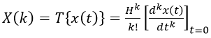
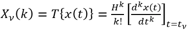
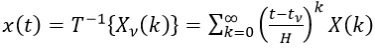
The original function is the continuous function x(t), which depends on the real parameter t, and the inverse function is the transform function X(k), which depends on the real integer argument k=0,1,2,…,∞. According to the definition of G.E. Pukhov [14], the transform DT of the function x(t) or the differential spectrum at   would be the following,

                                           (1)

Here H is the scale constant of the same size as the argument t . In general, if the  function is continuous everywhere, H=1, and if it is a piecewise-continuous function, it should be chosen separately for each interval [14]. If , then the series expansion of the function  would be the Maclaurin series and the differential spectra would be simpler,

                                                            (2)

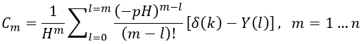
For, k=0,1,2,…,∞ , according to (1) and (2), differential spectra, which is, , ,…  can be easily calculated. According to these differential spectra, the original function  is obtained according to the following inverse formula:

                                         (3)

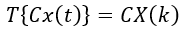
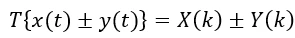
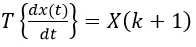
In general, the DT transform has many similar properties that are unique to all integral transforms. However, it is very important to consider the following main features in DT transform applications, both in solving differential equations and examining physical models [7,9–11,14,15]. C  is a constant, and in addition, the following (4) to (7) are given for any two analytic functions x(t)  and y(t) ;

                                                                (4)

                                                                                                (5)

                                                                                            (6)

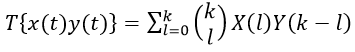                                                 (7)

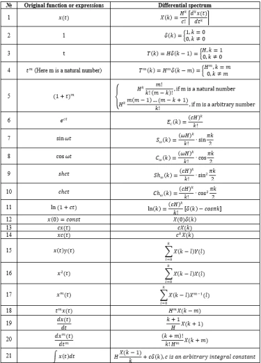
Unlike integral transform, the transform functions and operations of many functions, especially the convolution theorem in the DT transform, are determined by simpler algebraic expressions. This reveals that the DT transform is more advantageous than integral transforms in solving nonlinear equations and in modeling systems with varying parameters. . In this context, the basic principles and scientific foundations of the application of the DT transform to the solutions of many electro-technical problems have been studied in sufficient detail in the Pukhov books [11, 14, 15]. In this approach, the study of linear and non-linear electrical circuits and systems with distribution parameters was examined. The DT transforms of some important functions used in these applications are given in table A.1 in Appendix. DT transforms of more complex functions and equations are explained with problem solutions and table illustrations in Pukhov's books [7, 9– 11, 14, 15, 19].
By using table A.1, simpler solutions can be obtained by creating DT models of many nonlinear and variable coefficient differential equations. The most important advantage of this method is to obtain analytical (in the form of Taylor and non-Taylor series) and spectral numerical solutions from DT models.
However, this method, which seems straightforward in theory, is not advantageous in many practical applications. Since the convergence of the Taylor series in (3) is not fast enough in many cases, the calculation process becomes difficult, and the resulting calculation errors can reach undesirable levels. To eliminate these errors, G.E. Pukhov proposed the non-Taylor method, which is more effective by combining the X(k) differential spectra acquired by the DT method with different approximation methods (Picard's method, Newton-Kantorovich method, Poincare, Bubnov-Galerkin method, small square approximation, finite elements etc.) [7, 9– 11, 14, 15, 19]. Pukhov demonstrated that the GCM approach would be more effective in solving electro technical problems [8]. The presence of many process-specific properties in electrical circuits and systems (laws of commutation, stability, limited values of parameters such as current, voltage, magnetic flux in the circuit, etc.)  facilitates the creation of DT models of these problems. In the next part, we will discuss the creation of the DT model for some electro technical problems and the examination of simple transient regimes with the GCM. Examination of similar problems in every aspect is adequately covered in Pukhov's books [7, 9– 11, 14, 15, 19].

Differential transform and GCM

Let us assume that the state equation of the physical model or process to be examined is given as the following differential equation,

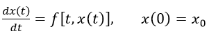                  (8)

The solution of this equation will generally be done with the following integral equation,

                      (9)

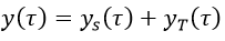
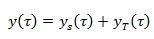
Here x(t) and f[t,x(t)] are the basis functions and x(0) is the initial value of the function x(t) for t=0. If (8) or (9) has only one solution, it can be assumed that the solution consists of two components,

                                             (10)

Here,  is the steady-state component and  is the temporary component [6–11,14,15,19]. In physical systems, the function of the system that stabilizes over time ( ) can be chosen as the steady-state component. This is a function that is independent on the initial time ( ). The steady-state function has limited amplitude, and its functional structure is the only one.

          In general, the steady-state component can be chosen to be approximately equal to one particular solution of the given equation. The analytical structure of the temporary component   must be chosen in such a way that the approximate function  representing this function is complete and damped. Here  are undetermined coefficients and are determined according to the initial and boundary conditions of the system or any other property. The DT method can be used to determine these coefficients. For this purpose, determination of differential spectra from (10) is required.

Let it be assumed that the DT spectrums of the  function are . Thus,  spectra [ , ,…, ] can be easily determined from (8) or (9). If it is desired to create the differential spectra of the functions according to the main differential equation of the physical process, then these spectra are determined from formulas or tables [7, 9– 11, 14, 15, 19].

The special conditions other than the physical properties of the nonlinear system (initial conditions, steady-state, etc.) are not required while (10) is being constructed. In other words, the detailed procedure of the solutions of the differential equations expressing the transient events system may not be taken into account. Moreover, when the DT transform is applied, the procedure followed for examining transient regimes in nonlinear systems can be similar to the procedure performed for examining transient regimes in linear systems. For this reason, this method was named the GCM by G.E. Pukhov [6– 11, 14, 15]. Many transient events in electrical circuits and systems can be easily examined when this method is applied.

Basic principles for analysis of electrical circuits by using DT transform

4.1. Creation of basic laws and elements of electrical circuits with DT models
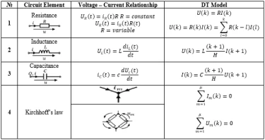
Basic laws of electrical circuits are Kirchhoff's laws the state equations of electrical circuit elements, and Maxwell's equations. In general, these equations are in the form of a specific ODE and PDE. DT models of Ohm-Kirchhoff's laws and circuit elements such as resistors, inductive windings, and capacitors are obtained as in table A.2 in Appendix [11, 14, 15].  In table A.2, where I(k)=T{i(t)}, U(k)=T{u(t)}, is the T model of current i(t)  and voltage u(t) respectively.
As can be seen from table A.2, Kirchhoff's first and second laws and Ohm's law provide their original shape in the DT transform, with R=constant. Since electrical circuit elements (resistance, inductance, and capacitance) can be linear or nonlinear, differential or integral relations express the voltage-current characteristics of these elements. Therefore, the expressions of these elements in the state equations of the electrical circuits should also be according to the DT transform.
In the following section, the GCM examines the changes in current and voltage on the nonlinear resistor R(t) in simplified RC, RL, and complex RLC electrical circuits.

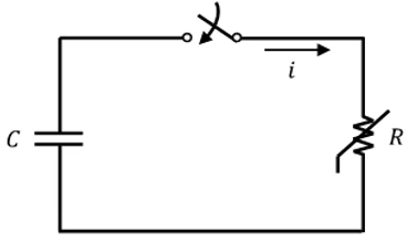
4.2. Examination of discharge events in nonlinear RC Electric Circuits by GCM
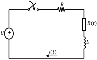
First of all, let's create the general model of the temporary regimes in simple nonlinear RC electric circuits using the DT transform on the basis of the GCM. As an illustration, the discharge event of the capacitor in the RC circuit with nonlinear resistance will be taken into consideration. In the circuit without current source shown in figure 1, the transient regime is determined as follows:

                            (11)

Figure 1. Transients in a simple nonlinear RC  electrical circuit: 

Full size image

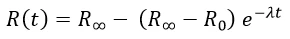
If it is assumed that the heat transfer between the resistor and the external environment is negligible during the transient regime, the amount of heat Q(t) generated on the resistor is completely spent on heating the resistor. In that case, if the limit resistance R(t) can reach in the case of t→∞ is assumed to be , the time change can be written as follows,

                      (12)

Here  is the time constant of the circuit and  is the initial value of the resistor. By taking the derivatives of (11) and (12), the state equation for the discharge event of the capacitor is obtained as follows.

                     (13)

Here  is the initial value of the current and,

       (14)

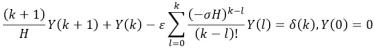
The nonlinear differential (13) allows examining the transient regime in the RC circuit including the nonlinear resistor R(t). This transient regime can be conveniently examined using the GCM [6, 7, 21– 29, 8– 11, 14, 15, 19, 20]. For the solution of these equations with the DT method, the DT spectrum model of (13) becomes as follows [6– 11, 14, 15]:

   (15)

According to the GCM created on the basis of DT, the solutions of (13) and (15), which express the state equation of the RC  circuit, can be written as follows,

                                   (16)

According to the characteristics of the problem examined, the following boundary conditions must be met in the solutions given in (16),

                        (17)

Therefore, the steady-state component for (16) would be as follows,

                                 (18)

The following criteria should be considered in determining the functional correlation of the temporal component :  and . Accordingly, the functional structure of the  temporary component can be as follows,

                          (19)

Here  are undetermined coefficients. The DT spectra of (15) are obtained for  as follows,

                 (20)

Considering the spectra of (20) at k = 0,1,⋯ values, the undetermined coefficients are as follows,

                                       (21)

                           (22)

                                                  (23)

Considering these coefficients, the approximate analytical solution of (13) is as follows,

               (24)

This expression expresses the dimensionless variation of the transient discharge current in a nonlinear RC circuit. The analytical solution of (13) is obtained as follows,

                           (25)

Figure 2. Variation of transient current in nonlinear  circuit

Full size image

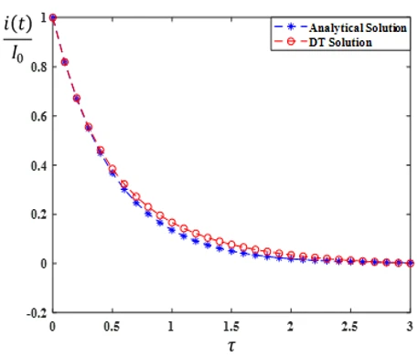
Comparison of the results from (24) and (25) is shown in figure 2. It is clearly seen that these results are similar. In order to reduce the difference error, it is necessary to increase the number of undetermined coefficients of the approximate function selected in (19) or to choose more convergent functions expressing transient regimes.

4.3. Examination of transient events in Nonlinear RL Electric Circuits by GCM
Suppose that the self-resistance of the inductivity R(t) in the simple electric circuit shows in figure 3 varies according to (12) and here  and U=constant.

Figure 3. Nonlinear  circuit

Full size image

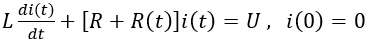
Let's examine the current change in transient events after the commutation, by using the GCM. In the transient events, the differential equation of the circuit is written as,

                            (26)

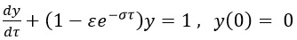
In dimensionless form, this equation becomes as given below,

     (27)

Here,

                (28)

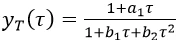
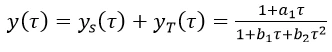
According to the GCM, the solution of (27) is written in dimensionless form as follows,

                    (29)

According to the character of transient events, . In this case,  and . When , the  temporal component can be selected as follows,

              (30)

Here ,  and  are undetermined coefficients. Therefore, the solution of (27) as follows,

            (31)

It would be better to write this equation as follows for constructing the DT model,

                             (32)

The T models of (27) and (32) are obtained as follows [7],

               (33)

                                  (34)

Since the p  coefficient here does not change the nature of the solution of the equation, this coefficient can be determined based on any special cases in the circuit. For example, the coefficient p  can be easily calculated according to the condition for  [7]. According to the calculations in (33) and (34), we find that,

                             (35)

The p>0  values are obtained from the following equation,

                             (36)

For example, for the values of , and , the transient current change in the nonlinear  circuit will be as follows according to (31),

                      (37)

The approximate solutions of the differential (26) of the nonlinear RL  circuit for different ε  values are shown in figure 4.

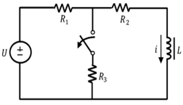
In many cases, the non-linear variation in the electrical circuit RL shown in figure 3 is given as a formula of magnetic flux-current relationships (ψ(i)) . These magnetic flux-current relationships can be given at different mathematical function forms such as exponent, harmonic sine (cosine), series or polynomials, etc. In this case, the current or voltage variations in the circuit can be easily solved by the GCM. For example, suppose that the RL circuit in figure 5 where the nonlinear magnetic flux-current relationship is given as 2 . Here  is the constant correction coefficient. At  in the circuit, the switch is opened and after the commutation event, the change of the current  in the transient event should be determined.

Figure 3. Nonlinear  circuit

Full size image

The variation of the current  in the transient event is determined by the following differential equation,

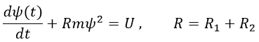                (38)

In this case, the variation of the current  with time is determined by the GCM as follows.  First, let's assume that the current in the circuit at time  is  According to the GCM, the general solution of (38) is assumed as following,

                            (39)

Figure 4. Transient current change in nonlinear  circuit

Full size image

The component is easily determined after the transient events  in the circuit,

                                        (40)

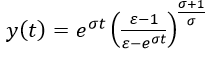
In this case, the determined steady current in the circuit will be as follows,

                                         (41)

Before the commutation event, due to the steady state in the circuit, the current at t = 0  is found as follows,

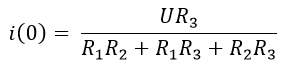                                   (42)

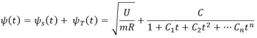
The transient component    contained in (39), can be selected as the following function,

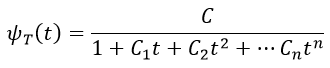                            (43)

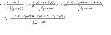
Here  are undetermined coefficients. As a result, the approximate solution of (38) is as follows,

             (44)

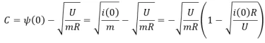
Since  at time , the constant  can be easily calculated,

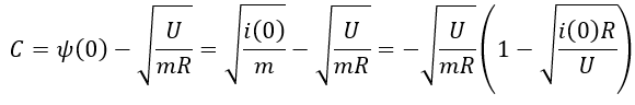           (45)

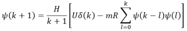
The remaining undetermined coefficients (  )   can be determined according to the following T models of (38) and (44).

                   (46)

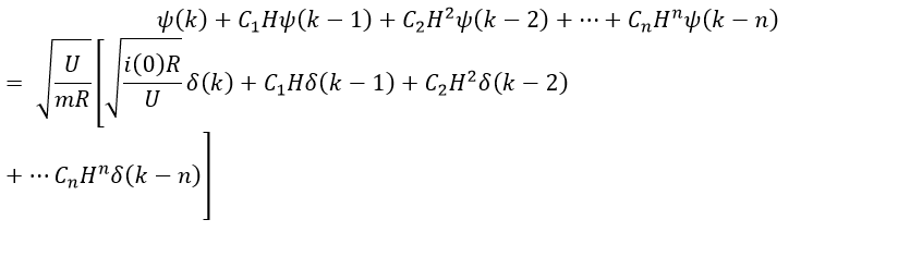(47)

Differential spectra are determined from the differential equation of the circuit from (46),

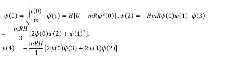(48)

Considering these spectra, the undetermined coefficients ( ) can be easily determined from (46).

(49)

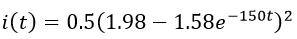
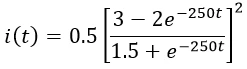
By using the coefficients can be determined an approximate analytical solution of (38). The transient current   in the circuit is calculated as . The solution of (36) obtained by GCM can be compared with the solutions given in the literature [29]. By using values circuit elements in the literature [29]: U=250 V,   for  was obtained that    and  . By using this data, the transient current  in the circuit has been obtained by different solving methods as follows [29]:

1. With approximate analytical solution;

                                        (50)

2. According to the linearization approach;

                (51)

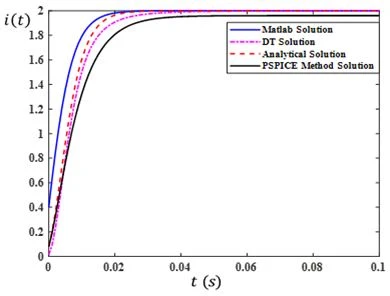
Figure 6. Results of solutions for variations transient current with different methods

Full size image

Figure 6 shows the graphs of the results obtained from (38), (50), and (51). According to these results, it is clearly seen that the result obtained with GCM is more compatible with the analytical solution than the other results. The GCM can be similarly applied to different voltage forms (harmonic, exponential, pulse, non-sinusoidal) of nonlinear electrical circuits.

Results and discussion

The transient regimes in AC and DC circuits with nonlinear components , , and  can be easily examined using differential transform method [10].In this case, it is possible to obtain approximate analytical and numerical solutions of the problem. The use of the GCM based on differential transform to investigate the state equation of transient events in electrical circuits and systems has many advantages. By using GCM, transient events in both linear and non-linear electrical circuits can be obtained without detailed procedures for solving the differential state equations of these circuits. In this case, the steady-state functions  and the transient functions  can be chosen as sufficiently convergent functions that satisfy the physical properties of the transient regimes in this circuit. Figure 2 shows the results of the variation of the capacitor discharge current in the nonlinear RC circuit according to the dimensionless time, calculated according to (13). The analytical solution of (13) is also shown on the graph for comparison. As can be seen from figure 2, the analytical and approximate solutions overlap each other. However, only three undetermined coefficients ( ) are used in (24) for the approximate solution obtained by the GCM. By increasing the number of terms with undetermined coefficients, can also increase the accuracy of the approximate solution.
Figure 4 shows that the normalized current in the circuit varies according to dimensionless time as a result of variations in the inductive windings self-resistance  with time for different  values. As can be seen from figure 4, the variation of the  resistance with time seriously affects the transient events in the circuit. This variation is often neglected in practical calculations.
In figure 6, the solution results of the time variation of the transient current in an  circuit with nonlinear inductance using the GCM are shown. These solution results are compared with different analytical and approximate solutions. As seen from the figure 6, the closest result to the analytical solution of the problem from all these methods is the approximate solution obtained by the GCM.
Therefore, these results show that the GCM has wider facilities than the traditional methods presented in the literature in the examination of transient events in both AC and DC non-linear electrical circuits.

Conclusion

The following results are obtained from the application of the GCM based on the differential Taylor (DT) transform to the analysis of transient events in nonlinear electrical circuits. The DT transform method is a spectral model created on the basis of the determination of differential spectra. This method was determined for the first time by the Ukrainian scientist G.E. Pukhov, and it was applied to the basic concepts and the solution of different mathematical problems, and the creation of physical models. 
The differential transform method is easier and more useful in practical applications than the integral transform methods commonly used in the literature. The results obtained by this method can be both numerically in the form of spectra and analytically in the form of an approximate serial or functional relationship.
The DT method is a more universal method that allows determining the original function in the form of different functions (non Taylor). In this respect, the Generalized Classic Method (GCM) created on DT ground in ODE or PDE solutions has wider facilities.
With the GCM, it is possible to consider the solution of transient events occurring in any dynamic system expressed with nonlinear ODE or PDE as a function consisting from steady state and temporary components. The steady-state component can be determined according to the steady state in the system. The temporary component can be chosen as an approximate function that satisfies the initial or boundary conditions or any other conditions in the system.
The GCM is a method with wide possibilities that allow to the examination of transient events occurring in both linear and non-linear electrical circuits with a similar procedure. If there is a steady-state regime in non-linear electric circuits and this solution is unique, then using the GCM, we can obtain the transient regimes in such electric circuits without solving the state equation (integro-differential equation) of the circuit.
The analysis of transient regimes realized in a simple nonlinear and linear RC, RL, and RLC electrical circuit with DT transform is shown. The results of the transient current or voltage changes in the circuit obtained by the GCM are in good agreement with the solutions presented in the literature with other approximate methods. In addition, GCM allows to obtain faster and more accurate results than other approximate solution methods. Therefore, the GCM can be used as an advantageous instrument for the study of transient events in more complex electrical circuits.

References

About this article